Netpicking Part 3: Prediction Sets
It’s been a while since I looked at mnistk. Recently, I came across this
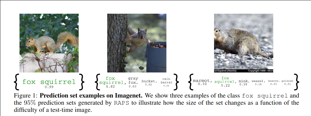
interesting paper which describes something
called Regularized Adaptive Prediction Sets (RAPS), a technique for
uncertainty estimation. The RAPS algorithm wraps a model’s prediction scores to
output a set that contains the true value with high probability for a given
confidence level $\alpha$. Basically, instead of getting a single class output
(“this image is a squirrel”), we can now get a set. See the example from the
paper:
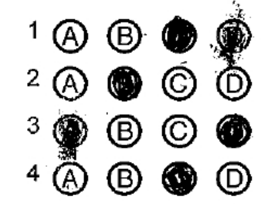
My original mnistk post used the analogy of an exam to select the best
network. Let’s continue with that here. If a single output is like filling in a
bubble in a multiple-choice test, then a prediction set output is like …
shoddily filling in multiple bubbles.
This post is about using RAPS to help me choose the best network from mnistk.
Getting the data
I implemented the RAPS algorithm for mnistk a while
back, but I didn’t get the time
to test it out. The RAPS algorithm requires a calibration dataset when
initializing the wrapper logic. I used the first 10000 samples from the QMNIST
dataset for calibration, and the
remaining 50000 samples as test data to obtain prediction sets. The original
mnistk networks had 1001 networks and 12 snapshots per network. That gives
1001 x 12 x 50000 = 600.6 million prediction set data to look at.
It took around 20 hours (on some AWS EC2 torch cpuonly system) to get this
data. I found that my implementation of the RAPS algorithm got a 2x
speedup if I did all the
torch neural network stuff first, and then used numpy vectorization to process
the scores for calibration and testing.
Plotting helps … but not much
Simple things first, let’s look at how prediction set size is related to accuracy:
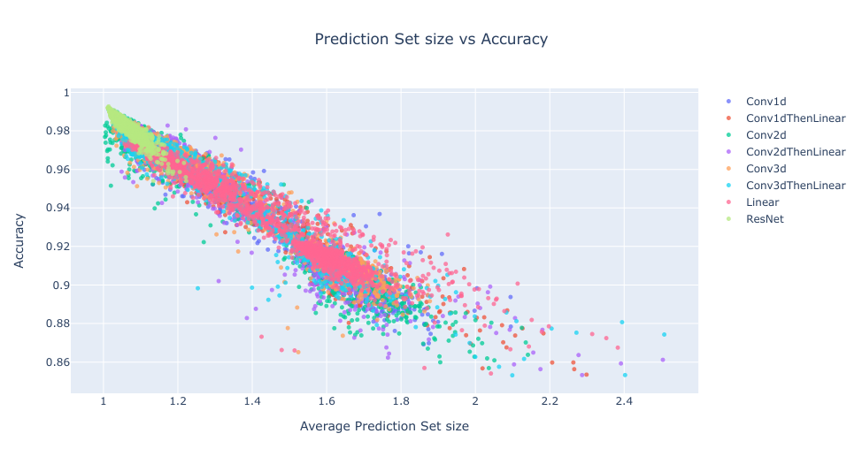
Okay, prediction set size seems to follow a linear-ish relationship to the accuracy of the network. I did a bunch of other plots similar to the ones in Part 1 which showed similar group characteristics. But these plots aren’t helping me as much with what I want: I want some metric to help me pick the best network.
Looking at the top 10
Let’s look at the top 10 networks in terms of accuracy: I’ll use num_c, the
number of correct answers (out of 50000). For simplicity, I picked the best
performing snapshot for each network, leaving us with 1001 entries.
| name | accuracy_rank | num_c |
|---|---|---|
| ResNetStyle_85 | 1 | 49636 |
| ResNetStyle_71 | 2 | 49610 |
| ResNetStyle_56 | 3 | 49599 |
| ResNetStyle_58 | 4 | 49597 |
| ResNetStyle_69 | 5 | 49582 |
| ResNetStyle_81 | 6 | 49572 |
| ResNetStyle_89 | 7 | 49569 |
| Conv2dReLU_14 | 8 | 49558 |
| ResNetStyle_66 | 9 | 49552 |
| ResNetStyle_83 | 10 | 49544 |
As expected, ResnetStyle models dominate. But the above scatterplot said
prediction set sizes are closely related to accuracy. Let’s call a prediction
with only one element in the prediction set as a sure prediction. Let’s look
at the top 10 networks in terms of num_s the number of predictions about which
they are sure:
| name | accuracy_rank | num_s | num_c |
|---|---|---|---|
| Conv2dSELU_6 | 136 | 49568 | 49212 |
| ResNetStyle_58 | 4 | 49498 | 49597 |
| ResNetStyle_71 | 2 | 49442 | 49610 |
| ResNetStyle_56 | 3 | 49440 | 49599 |
| ResNetStyle_81 | 6 | 49425 | 49572 |
| Conv2dReLU_14 | 8 | 49383 | 49558 |
| ResNetStyle_85 | 1 | 49379 | 49636 |
| ResNetStyle_47 | 11 | 49337 | 49541 |
| ResNetStyle_89 | 7 | 49321 | 49569 |
| ResNetStyle_88 | 33 | 49319 | 49497 |
Where did Conv2dSELU_6 come from!? Somehow it is dominating in terms of
minimal prediction set size. If I deployed this model in the real world, I would
rarely see any uncertainty reported along with its predictions. But it is not in
the top 10 for accuracy; in fact its rank is 136, nowhere close to the top, so
from where is it getting all that confidence?
Alright, best of both worlds. I want a model that not only gets a lot of answers
correct, but also is sure (highly confident) about the correct answers it gets.
Let’s look at the top 10 networks in terms of num_cs, the number of correct
answers in which they are sure:
| name | accuracy_rank | num_c | num_s | num_cs |
|---|---|---|---|---|
| ResNetStyle_58 | 4 | 49597 | 49498 | 49306 |
| ResNetStyle_56 | 3 | 49599 | 49440 | 49260 |
| ResNetStyle_71 | 2 | 49610 | 49442 | 49258 |
| ResNetStyle_85 | 1 | 49636 | 49379 | 49237 |
| ResNetStyle_81 | 6 | 49572 | 49425 | 49211 |
| Conv2dReLU_14 | 8 | 49558 | 49383 | 49181 |
| ResNetStyle_47 | 11 | 49541 | 49337 | 49128 |
| ResNetStyle_89 | 7 | 49569 | 49321 | 49127 |
| ResNetStyle_92 | 20 | 49526 | 49272 | 49090 |
| ResNetStyle_88 | 33 | 49497 | 49319 | 49087 |
Now the top 10 is seeing some shakeups! The original “best” network is sometimes not sure when being correct, so it falls down the rankings. What happens when the model’s predictions are wrong (don’t match with ground truth) or the model is unsure about the predictions (set size is greater than 1)?
Each prediction made by the model can fall into one of four classes:
| sure | unsure | total | |
|---|---|---|---|
| correct | num_cs | num_cu | num_c |
| wrong | num_ws | num_wu | num_w |
| total | num_s | num_u | 50000 |
num_cs-> the model guessed correctly, and prediction size is 1. Ideally, all the model’s predictions would be here.num_cu-> the model guessed correctly, but the prediction set size is greater than 1. This means the model’s prediction still has a nonzero chance of being something else. These predictions are okay, but not as reassuring asnum_cs, and may require a second look. Ideally,num_cswould be zero, a high value indicates this model needs confirmation checks quite frequently.num_ws-> the model guessed wrongly, and prediction size is 1. This means the model is sure about a prediction that does not match the ground truth. These predictions are bad, because the confidence means the prediction will not be second-guessed. Ideally,num_wswould be zero, but a non-zero value may indicate some difficult samples or incorrectly labeled data.num_wu-> the model guessed wrongly, the prediction set size is greater than 1, and the correct answer does not appear in the prediction set. These predictions are bad, but not as bad asnum_ws, because they indicate a second check might be needed. However, the issue is when the backup check can return an answer that is not there in the prediction set, which may cause confusion.
Hmm num_wu indicates there is a fifth class of predictions:
num_we-> the model guessed wrongly, the prediction set size is greater than 1, but the correct answer exists in the prediction set. These predictions are weird, because the backup check will resolve the uncertainty, so why are they made in the first place? Why is the correct answer hiding in the prediction set instead of being the first guess?
Let’s look at the top 10 again with these five quantities:
| name | accuracy_rank | num_cs | num_cu | num_ws | num_wu | num_we | num_sum5 |
|---|---|---|---|---|---|---|---|
| ResNetStyle_58 | 4 | 49306 | 291 | 192 | 29 | 182 | 50000 |
| ResNetStyle_56 | 3 | 49260 | 339 | 180 | 21 | 200 | 50000 |
| ResNetStyle_71 | 2 | 49258 | 352 | 184 | 25 | 181 | 50000 |
| ResNetStyle_85 | 1 | 49237 | 399 | 142 | 25 | 197 | 50000 |
| ResNetStyle_81 | 6 | 49211 | 361 | 214 | 23 | 191 | 50000 |
| Conv2dReLU_14 | 8 | 49181 | 377 | 202 | 29 | 211 | 50000 |
| ResNetStyle_47 | 11 | 49128 | 413 | 209 | 32 | 218 | 50000 |
| ResNetStyle_89 | 7 | 49127 | 442 | 194 | 23 | 214 | 50000 |
| ResNetStyle_92 | 20 | 49090 | 436 | 182 | 37 | 255 | 50000 |
| ResNetStyle_88 | 33 | 49087 | 410 | 232 | 36 | 235 | 50000 |
How can we use the information about the models’ less-than-ideal predictions
(everything except num_cs) to find the best network? Keeping with the analogy,
we can have negative marking, that nasty troll from competitive
exams.
First let’s subtract a mark for each unsure or incorrect answer:
| name | accuracy_rank | cs - all | num_cs | num_cu | num_ws | num_wu | num_we |
|---|---|---|---|---|---|---|---|
| ResNetStyle_58 | 4 | 48612 | 49306 | 291 | 192 | 29 | 182 |
| ResNetStyle_56 | 3 | 48520 | 49260 | 339 | 180 | 21 | 200 |
| ResNetStyle_71 | 2 | 48516 | 49258 | 352 | 184 | 25 | 181 |
| ResNetStyle_85 | 1 | 48474 | 49237 | 399 | 142 | 25 | 197 |
| ResNetStyle_81 | 6 | 48422 | 49211 | 361 | 214 | 23 | 191 |
| Conv2dReLU_14 | 8 | 48362 | 49181 | 377 | 202 | 29 | 211 |
| ResNetStyle_47 | 11 | 48256 | 49128 | 413 | 209 | 32 | 218 |
| ResNetStyle_89 | 7 | 48254 | 49127 | 442 | 194 | 23 | 214 |
| ResNetStyle_92 | 20 | 48180 | 49090 | 436 | 182 | 37 | 255 |
| ResNetStyle_88 | 33 | 48174 | 49087 | 410 | 232 | 36 | 235 |
That didn’t change the order at all, so let’s have weighted negative marking.
- Being sure about a wrong answer (
num_ws) is clearly the worst thing to do, gets a weight of … let’s say 12. - Being unsure about a wrong answer but not considering the correct answer (
num_wu) gets a weight of 9. - Being unsure about a wrong answer but at least considering the correct answer (
num_we) gets a weight of 8. - Being unsure about a correct answer (
num_cu) gets a weight of 6.
Now let’s see if the top 10 shift:
| name | accuracy_rank | cs - weighted | num_cs | num_cu | num_ws | num_wu | num_we |
|---|---|---|---|---|---|---|---|
| ResNetStyle_58 | 4 | 43539 | 49306 | 291 | 192 | 29 | 182 |
| ResNetStyle_85 | 1 | 43338 | 49237 | 399 | 142 | 25 | 197 |
| ResNetStyle_56 | 3 | 43277 | 49260 | 339 | 180 | 21 | 200 |
| ResNetStyle_71 | 2 | 43265 | 49258 | 352 | 184 | 25 | 181 |
| ResNetStyle_81 | 6 | 42742 | 49211 | 361 | 214 | 23 | 191 |
| Conv2dReLU_14 | 8 | 42546 | 49181 | 377 | 202 | 29 | 211 |
| ResNetStyle_89 | 7 | 42228 | 49127 | 442 | 194 | 23 | 214 |
| ResNetStyle_47 | 11 | 42110 | 49128 | 413 | 209 | 32 | 218 |
| ResNetStyle_69 | 5 | 41998 | 49075 | 507 | 167 | 23 | 228 |
| ResNetStyle_92 | 20 | 41917 | 49090 | 436 | 182 | 37 | 255 |
Indeed they did: the overall rankings shifted, and a network from the original
top 10 (ResnetStyle_69) sneaked back in because of the new scoring scale. Of
course, the weights I picked were arbitrary, but the point is that the
incorrect/unsure predictions also need to considered when trying to choose the
best network.
Closing Notes
Regularized Adaptive Prediction Sets (RAPS) provide additional context when I
need to choose the best network. Earlier, I could examine networks in terms of
accuracy/weights/memory use/training time. Now, with surface-level information
about the prediction sets (just set sizes), I can break down a raw accuracy
score into 5 different components, and choose the best network for my use case
by assigning weights for the types of errors I don’t want. This can be useful in
deployment: I am fine with networks on embedded devices having confidence issues
about predictions (especially for incorrect predictions). But complex networks
in the cloud should provide more confidence, because they are usually the last
resort. I am not certain (!) about what should be done when the initial
prediction is unsure, and the backup gives a different answer (the num_wu
case) because that seems ripe for confusion.
There are other interesting angles to examine. I want to see why that
Conv2dSELU_6 has so much confidence, and what means for the individual
predictions it makes. The RAPS algorithm provides two hyperparameters, $k$ and
$\lambda$ in addition to $\alpha$, and a wrapper to find the optimal $k$ and
$\lambda$ for a given network during calibration. I used the same $k$ and
$\lambda$ values throughout, so that leaves me to wonder how much the above
tables are affected if I use the optimal values. I have also not used the
calibrated scores or the generalized quantile values anywhere in the analysis.
That’s probably worth a separate round on AWS and another post.